10 Ch 2 - SLR
In the second part of your BP you will have chapters for most of the main econometrics / statistics topics we cover. This chapter is on simple linear regression (SLR), i.e., regression with 1 explanatory variable. This should be review from STAT 255, so it is simply a few examples to replicate to refresh your memory and make sure you can do these things in R. The second-level headings (i.e., those with 2 hash tags that show up in the navigation bar of the html files) in each file are labeled with the examples you should replicate from chapter 2 of the Wooldridge textbook. The data is loaded for you using the the wooldridge package (the wooldridge package has datasets from Wooldridge Introductory Econometrics 6th edition). I also suggest that you add notes on each chapter, but doing so is optional (except if I specify that notes are required).
For this chapter, you should do the simple linear regressions from the examples. For each, you should make sure you get the same results as in the example and understand the discussion of the example in the textbook. You should also use ggplot to create a scatter plot of the x and y variables used in the regression, and include a linear regression (lm) line, so you might want to do this chapter after you complete the DataCamp course and your notes on Intro to Data Visualization with ggplot2. For this chapter, you will also write a sentence that displays the values of the coefficient, standard error, t-stat, p-value, and the widest standard (i.e., 90%, 95%, 99%) confidence interval that does not include 0. This reminds you of how to calculate the t-stat and p-value from the coefficient and standard error, and the confidence interval using the critical value from the t-distribution. This also gives you practice with how to display calculated values in text sentences (i.e., outside of code chunks), a crucial R skill for reproducible research.
Note that in this chapter, you do not need to interpret the regression results or discuss them at all. We will go through in the next chapter the specific way you must interpret regression results for 380. We’ll wait for the next chapter when we have more than one explanatory variable.
These are the packages you will need:
## ── Attaching core tidyverse packages ──────────────────────── tidyverse 2.0.0 ──
## ✔ dplyr     1.1.4     ✔ readr     2.1.4
## ✔ forcats   1.0.0     ✔ stringr   1.5.1
## ✔ ggplot2   3.4.4     ✔ tibble    3.2.1
## ✔ lubridate 1.9.3     ✔ tidyr     1.3.0
## ✔ purrr     1.0.2
## ── Conflicts ────────────────────────────────────────── tidyverse_conflicts() ──
## ✖ dplyr::filter() masks stats::filter()
## ✖ dplyr::lag()    masks stats::lag()
## ℹ Use the conflicted package (<http://conflicted.r-lib.org/>) to force all conflicts to become errorslibrary(pander)
## datasets are in this package:
library(wooldridge)
## for visualizing t-stats and p-values on a t-distribution
library(ggformula)## Loading required package: scales
##
## Attaching package: 'scales'
##
## The following object is masked from 'package:purrr':
##
## discard
##
## The following object is masked from 'package:readr':
##
## col_factor
##
## Loading required package: ggridges
##
## New to ggformula? Try the tutorials:
## learnr::run_tutorial("introduction", package = "ggformula")
## learnr::run_tutorial("refining", package = "ggformula")For displaying the results of a single regression, you should use the pander package as shown in example 2.3 below. (Later in 380 you will be comparing several regression models side-by-side and will be using the stargazer package instead, but for a single regression model this works well).
I completed the first example (Example 2.3: CEO Salary and Return on Equity) for you to demonstrate what you need to do. For the subsequent examples you should fill in the code yourself. I’ve provided the template for you and included the code to load the data. I then added a comment that says “YOUR CODE GOES HERE” wherever you are supposed to add code (note that this is often in a code chunk as a comment, but for the sentence that’s outside a code chunk, it’s an html comment and won’t display in the book when you build it the way code chunk comments do). You should use the example I did for you as a guide. What you do later in 380 will not be as simple as copy/pasting code I give you and changing a few variable names, but for for this chapter, it’s exactly that easy. Don’t overthink what you’re being asked to do.
That said, you are of course welcome to add more if it will help you. You can add more regressions. You can explore the changes of units I talk about in LN2.7. You can experiment with log transformations shown in the later parts of chapter 2 (we’ll talk about these later with chapter 3). But the only things you’re required to do for the BP are the 2 examples I left for you below.
10.2 Example 2.3: CEO Salary and Return on Equity
Load the data from wooldridge package, estimate the regression, and display the results
# Load data
data(ceosal1)

# Estimate regression model
ex2.3 <- lm(salary ~ roe, data=ceosal1)

# Display model results
pander(summary(ex2.3))| Estimate | Std. Error | t value | Pr(>|t|) | |
|---|---|---|---|---|
| (Intercept) | 963.2 | 213.2 | 4.517 | 0.00001053 |
| roe | 18.5 | 11.12 | 1.663 | 0.09777 |
| Observations | Residual Std. Error | \(R^2\) | Adjusted \(R^2\) |
|---|---|---|---|
| 209 | 1367 | 0.01319 | 0.008421 |
Display a scatter plot with regression line corresponding to this model
## `geom_smooth()` using formula = 'y ~ x'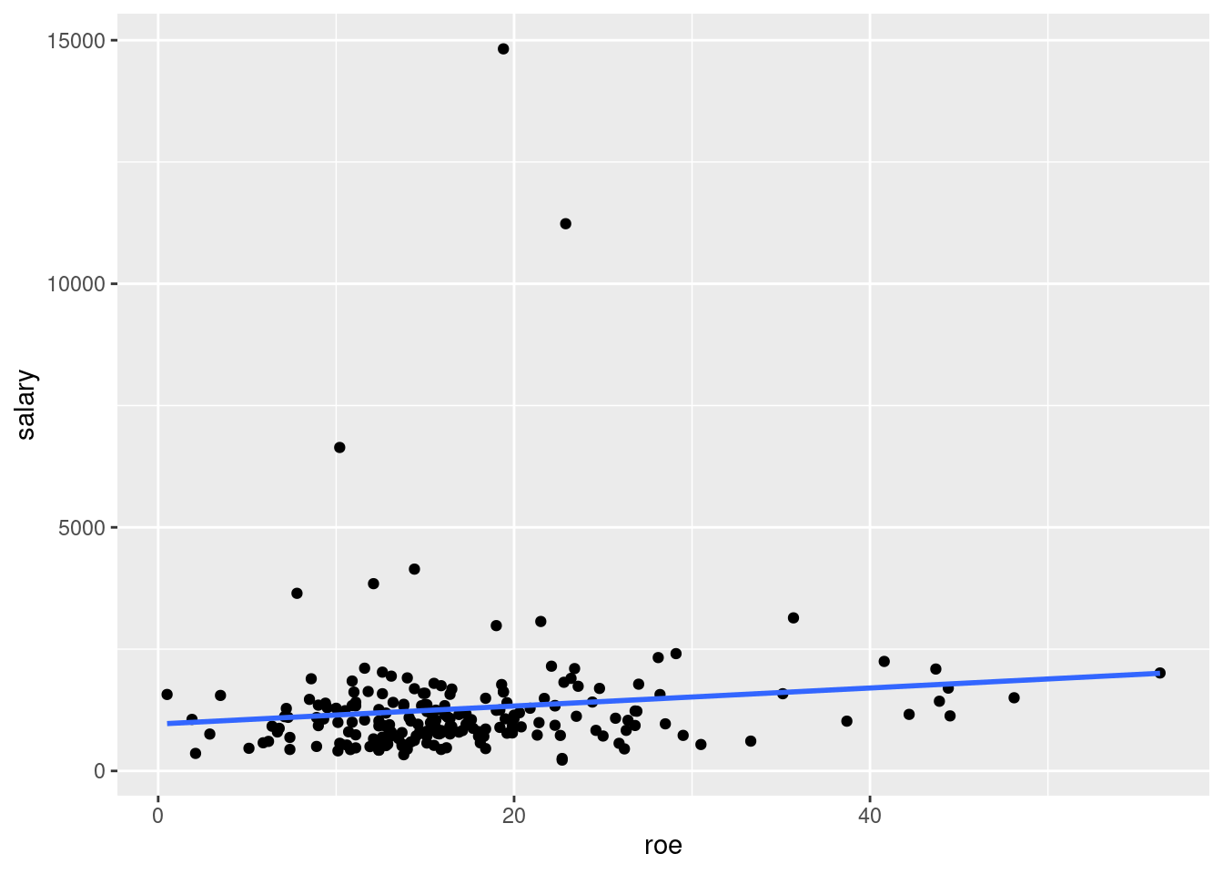
10.2.1 T-stats, p-values, and statistical significance
Later in the course we will often be displaying regression results for multiple models side-by-side. For tables that report the results of multiple models, there is not sufficient space to display everything we see in the regression output above. Obviously we display the coefficients, but we also have to choose one of the measures of uncertainty associated with the coefficients to display as well. For this course, we will typically display p-values.
There is not one standard used in economics for what should be displayed to convey the uncertainty of the coefficients. Some authors choose to display p-values, some t-statistics, some standard errors, and some confidence intervals. The same is true for journal articles in many disciplines, and other places you see statistical results reported. Thus, it is important to understand not just p-values, but also standard errors, t-stats, and confidence intervals.
Here, we will walk through how to manually calculate t-stats and the associated p-values. This should also help you see how standard errors relate to t-stats and p-values, and, in turn, to the concept of statistical significance (and the *’s you often see in journal articles).
These calculations work the same way with multiple regression. We are examining it here because with only one explanatory variable we are displaying output using pander. This displays the coefficient, standard error, t-stat, and p-value, so you can easily see if you have calculated the t-stat and p-value correctly. Typically you do not need to calculate t-stats, p-values. and confidence intervals manually, but it is important to understand how to do so because that helps you understand what they are and what they communicate about the uncertainty of the associated regression coefficients.
There are many ways in R to access the coefficient and standard error from a regression model (lm) object. Below is one way, but you are free to access these values however you want.
# Coefficients are accessed via the coef function, with square brackets to get the specific coefficient by name
coef <- coef(ex2.3)["roe"]
coef
## roe
## 18.50119# The standard errors are accessible via the summary of the model:
se <- summary(ex2.3)$coefficients["roe","Std. Error"]
se## [1] 11.12325## Note that you can also get the coefficient using summary, i.e., summary(ex2.3)$coefficients["roe","Estimate"]
## ...but it is usually easier to use coef(ex2.3)["roe"] instead
# The t-stat is the coefficient divided by the standard error
tStat <- coef/se
tStat## roe
## 1.663289# The degrees of freedom for the t-distribution are obtained from the model summary:
dof <- summary(ex2.3)$df[2]
dof## [1] 207# Note that the degrees of freedom are equal to the number of observations, minus the number of things that were estimated:
nobs(ex2.3) - length(coef(ex2.3))## [1] 207# To find the p-value, find the probability of getting a t-stat no larger (in the left tail) than our tStat,
# and multiply it by 2 to make it 2 tailed
pValue <- 2*pt(-abs(tStat),dof)
pValue## roe
## 0.09776775Now lets also calculate the standard confidence intervals, by which we mean the 90%, 95%, and 99% confidence intervals.2 We can first use confint and display the results using pander. Then we will manually calculate the confidence interval for the slope coefficient. You will need to display one of the confidence intervals as part of the sentence you must display for each example (specifically, the widest of the standard confidence intervals that does not include 0).
90% confidence interval:
| 5 % | 95 % | |
|---|---|---|
| (Intercept) | 610.9 | 1316 |
| roe | 0.1228 | 36.88 |
##       roe
## 0.1228163## roe
## 36.8795695% confidence interval:
| 2.5 % | 97.5 % | |
|---|---|---|
| (Intercept) | 542.8 | 1384 |
| roe | -3.428 | 40.43 |
##       roe
## -3.428196## roe
## 40.4305799% confidence interval:
| 0.5 % | 99.5 % | |
|---|---|---|
| (Intercept) | 408.8 | 1518 |
| roe | -10.42 | 47.42 |
##       roe
## -10.41691## roe
## 47.41928From what you’ve learned in STAT 255, you should understand the following about the above confidence intervals:
why the
panderoutput of theconfintconfidence intervals displays 5% and 95% for the 90% confidence interval, 2.5% and 97.5% for the 95% confidence interval, and 0.5% and 99.5% for the 99% confidence intervalwhy the 90% confidence interval is narrowest and the 99% confidence interval is widest (with the 95% confidence interval in the middle)
why, based on the p-value calculated above, the 90% confidence interval does not include 0, but the 95% and 99% confidence intervals do
If you do not understand any of these things, or how to calculate the confidence intervals manually, please review3 and ask any questions you have.
Finally, lets visualize the t-distribution with the t-stat and associated p-values.
gf_dist("t", df=dof, geom = "area", fill = ~ (abs(x)< abs(tStat)), show.legend=FALSE) + geom_vline(xintercept=c(tStat, -tStat), color="red")  + xlab("t") +
    annotate(
    "text",
    x = 3.5, y = 0.176,
    label = paste0("t = ", format(abs(tStat),digits = 3, nsmall=3)),
    vjust = 1, size = 3, color = "red"
  ) +
  annotate(
    "segment",
    x = 3., y = 0.17,
    xend = 1.75, yend = 0.17,
    arrow = arrow(length = unit(0.2, "cm"), type = "closed"),
    color = "grey40"
  ) +
    annotate(
    "text",
    x = 3, y = 0.12,
    label = paste0("Prob t > ", format(abs(tStat),digits = 3, nsmall=3), " = ", format(pValue/2,digits = 3, nsmall=3)),
    vjust = 1, size = 3, color = "red"
  ) +
  annotate(
    "segment",
    x = 3, y = 0.105,
    xend = 2.4, yend = 0.03,
    arrow = arrow(length = unit(0.2, "cm"), type = "closed"),
    color = "grey40"
  ) +
    annotate(
    "text",
    x = -3.5, y = 0.176,
    label = paste0("t = ", format(-abs(tStat),digits = 3, nsmall=3)),
    vjust = 1, size = 3, color = "red"
  ) +
  annotate(
    "segment",
    x = -3., y = 0.17,
    xend = -1.75, yend = 0.17,
    arrow = arrow(length = unit(0.2, "cm"), type = "closed"),
    color = "grey40"
  ) +
    annotate(
    "text",
    x = -3, y = 0.12,
    label = paste0("Prob t < ", format(-abs(tStat),digits = 3, nsmall=3), " = ", format(pValue/2,digits = 3, nsmall=3)),
    vjust = 1, size = 3, color = "red"
  ) +
  annotate(
    "segment",
    x = -3, y = 0.105,
    xend = -2.4, yend = 0.03,
    arrow = arrow(length = unit(0.2, "cm"), type = "closed"),
    color = "grey40"
  ) +
    annotate(
    "text",
    x = 0, y = 0.2,
    label = paste0("Prob t is between\n", format(-abs(tStat),digits = 3, nsmall=3), " and ", format(abs(tStat),digits = 3, nsmall=3), " = ", format(1-pValue,digits = 3, nsmall=3)),
    vjust = 1, size = 3, color = "black"
  )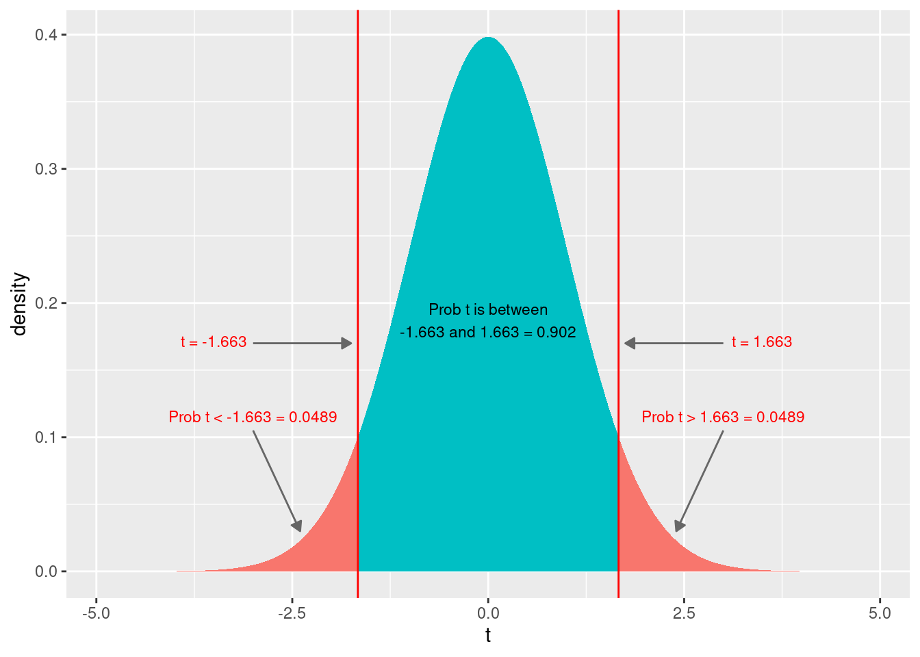
The t-stat tells us how many standard errors away from 0 our coefficient is. Recall that the formula for the t-stat is: \[ t_{\hat{\beta_j}} = \frac{\hat{\beta_j}-\beta_j}{SE(\hat{\beta_j})} \] where \(\hat{\beta_j}\) is our estimated coefficient, \(SE(\hat{\beta_j})\) is the standard error of our estimated coefficient, and \(\beta_j\) is the unknown true coefficient about which we have a null hypothesis. Recall that the most common null hypothesis is that the true coefficient is 0. That is, the null hypothesis is that the \(\beta_j=0\), i.e., that variable \(x_j\) has no effect on \(y\). This null hypothesis is so common that most regression packages report the t-stat and p-value associated with this hypothesis. Thus, the t-stat column is calculated: \[ t_{\hat{\beta_j}} = \frac{\hat{\beta_j}-\beta_j}{SE(\hat{\beta_j})} = \frac{\hat{\beta_j}-0}{SE(\hat{\beta_j})} = \frac{\hat{\beta_j}}{SE(\hat{\beta_j})} \] In other words, the t-stat is calculated by dividing the estimated coefficient by its standard error. Intuitively, this gives us how many standard errors away from 0 our estimated coefficient is. A larger coefficient for a given standard error, or, similarly, a smaller standard error for a given coefficient, is more standard errors away from 0, and, thus, is less likely to happen if the null hypothesis of \(\beta_j=0\) is true. At some point, our estimate is sufficiently far away from 0 in terms of standard errors (i.e., the t-statistic is large enough in magnitude) that we reject \(\beta_j = 0\), i.e., conclude that there is a relationship between variable \(x_j\) and y.
Looking at the t-distribution graphically above, we see the value of the t-stat, both on the left tail and the right tail (in absolute value). We see the probability of getting a t-stat lower than the value in the left tail, and the (identical) probability of getting a t-stat higher than the value in the right tail. Adding those two probabilities gives us the p-value. In other words, the p-value is the probability of getting a coefficient this extreme or more if the null hypothesis of no effect is true (i.e., if the true coefficient is \(\beta_j=0\)).
For some additional intuition, think about what would happen if the coefficient were larger in magnitude for a given standard error. The t-stat would increase in magnitude. Graphically, the vertical red lines would shift further out in the tails, leaving more room in between the two lines and less in the tails, i.e., a lower p-value.
In the examples below, you will need to estimate the regression, display a scatter plot, and write out a sentence explaining how to calculate the t-stat and p-value from the coefficient and standard error, and that also includes the widest standard confidence interval that does not include 0 calculated from the coefficient, standard error, and critical value. This also gives you practice with displaying regression results in sentences, You must do this without manually hard-coding the value into the text. This is part of writing reproducible research–if the regression results change, your sentence will update automatically.
Here is the sentence you should write for each example below:
The t-stat is calculated by dividing the estimated coefficient (18.501) by its standard error (11.123), yielding a t-stat of 1.663 and an associated p-value of 0.0978; the widest standard confidence interval that does not include 0 is the 90% confidence interval: (0.123, 36.880).
Obviously you need to adjust the code in the sentence above for each model. Make sure to display the correct confidence interval, both the displayed level and the confidence interval itself (in the sentence above, the level displayed is 90%, but you may need to change that for the other examples); it should be the widest of the standard confidence intervals that does not include 0 (yes, at least one of the standard confidence intervals does not include 0 for each example). Then make sure that the values match with the regression and confint output (i.e., look at the values in the pander output table and the sentence after you build your book and make sure they are the same). In the next chapter you will comment on statistical significance, but for here, this sentence is sufficient. Make sure you understand it, and ask questions if you do not.
10.3 Example 2.4: Wage and Education
Load the data from wooldridge package, estimate the regression, and display the results
# Load data
data(wage1)

# Estimate regression model
ex2.4 <-  lm(wage ~ educ, data = wage1)

# Display model results
pander(summary(ex2.4))| Estimate | Std. Error | t value | Pr(>|t|) | |
|---|---|---|---|---|
| (Intercept) | -0.9049 | 0.685 | -1.321 | 0.1871 |
| educ | 0.5414 | 0.05325 | 10.17 | 2.783e-22 |
| Observations | Residual Std. Error | \(R^2\) | Adjusted \(R^2\) |
|---|---|---|---|
| 526 | 3.378 | 0.1648 | 0.1632 |
Display the widest standard (i.e., 90%, 95%, or 99%) confidence interval for \(\hat{\beta_1}\) that does not include 0 (use pander and confint, and it’s fine that it also displays the same level confidence interval for \(\hat{\beta_0}\)):
# Coefficients are accessed via the coef function, with square brackets to get the specific coefficient by name
coef2.4 <- coef(ex2.4)["educ"]
coef2.4
## educ
## 0.5413593# The standard errors are accessible via the summary of the model:
se2.4 <- summary(ex2.4)$coefficients["educ","Std. Error"]
se2.4## [1] 0.05324804## Note that you can also get the coefficient using summary, i.e., summary(ex2.3)$coefficients["roe","Estimate"]
## ...but it is usually easier to use coef(ex2.3)["roe"] instead
# The t-stat is the coefficient divided by the standard error
tStat2.4 <- coef2.4/se2.4
tStat2.4## educ
## 10.16675# The degrees of freedom for the t-distribution are obtained from the model summary:
dof2.4 <- summary(ex2.4)$df[2]
dof2.4## [1] 524# Note that the degrees of freedom are equal to the number of observations, minus the number of things that were estimated:
nobs(ex2.4) - length(coef(ex2.4))## [1] 524# To find the p-value, find the probability of getting a t-stat no larger (in the left tail) than our tStat,
# and multiply it by 2 to make it 2 tailed
pValue2.4 <- 2*pt(-abs(tStat2.4),dof2.4)
pValue2.4## educ
## 2.782599e-22| 0.5 % | 99.5 % | |
|---|---|---|
| (Intercept) | -2.676 | 0.866 |
| educ | 0.4037 | 0.679 |
##      educ
## 0.4037001## educ
## 0.6790184Display a scatter plot with regression line corresponding to this model
## `geom_smooth()` using formula = 'y ~ x'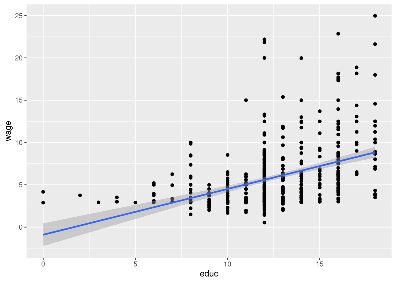
For \(\hat{\beta_1}\), display a sentence explaining how to calculate the t-stat and associated p-value, and displaying the widest standard (i.e., 90%, 95%, or 99%) confidence interval that does not contain 0 (with all values coming from inline r code, modeled after the sentence above for example 2.3):
The t-stat is calculated by dividing the estimated coefficient (0.541) by its standard error (0.0532), yielding a t-stat of 10.167 and an associated p-value of 2.78e-22; the widest standard confidence interval that does not include 0 is the 99% confidence interval: (0.404, 0.679).
10.4 Example 2.5: Voting Outcomes and Campaign Expenditures
Load the data from wooldridge package, estimate the regression, and display the results
# Load data
data(vote1)

# Estimate regression model
ex2.5 <-  lm(voteA ~ shareA, data = vote1)
# Display model results
pander(summary(ex2.5))| Estimate | Std. Error | t value | Pr(>|t|) | |
|---|---|---|---|---|
| (Intercept) | 26.81 | 0.8872 | 30.22 | 1.729e-70 |
| shareA | 0.4638 | 0.01454 | 31.9 | 6.634e-74 |
| Observations | Residual Std. Error | \(R^2\) | Adjusted \(R^2\) |
|---|---|---|---|
| 173 | 6.385 | 0.8561 | 0.8553 |
Display the widest standard (i.e., 90%, 95%, or 99%) confidence interval for \(\hat{\beta_1}\) that does not include 0 (use pander and confint, and it’s fine that it also displays the same level confidence interval for \(\hat{\beta_0}\)):
# Coefficients are accessed via the coef function, with square brackets to get the specific coefficient by name
coef2.5 <- coef(ex2.5)["shareA"]
coef2.5
## shareA
## 0.4638269# The standard errors are accessible via the summary of the model:
se2.5 <- summary(ex2.5)$coefficients["shareA","Std. Error"]
se2.5## [1] 0.01453965## Note that you can also get the coefficient using summary, i.e., summary(ex2.3)$coefficients["roe","Estimate"]
## ...but it is usually easier to use coef(ex2.3)["roe"] instead
# The t-stat is the coefficient divided by the standard error
tStat2.5 <- coef2.5/se2.5
tStat2.5## shareA
## 31.90083# The degrees of freedom for the t-distribution are obtained from the model summary:
dof2.5 <- summary(ex2.5)$df[2]
dof2.5## [1] 171# Note that the degrees of freedom are equal to the number of observations, minus the number of things that were estimated:
nobs(ex2.5) - length(coef(ex2.5))## [1] 171# To find the p-value, find the probability of getting a t-stat no larger (in the left tail) than our tStat,
# and multiply it by 2 to make it 2 tailed
pValue2.5 <- 2*pt(-abs(tStat2.5),dof2.5)
pValue2.5## shareA
## 6.63384e-74| 0.5 % | 99.5 % | |
|---|---|---|
| (Intercept) | 24.5 | 29.12 |
| shareA | 0.426 | 0.5017 |
##    shareA
## 0.4259528## shareA
## 0.501701Display a scatter plot with regression line corresponding to this model
## `geom_smooth()` using formula = 'y ~ x'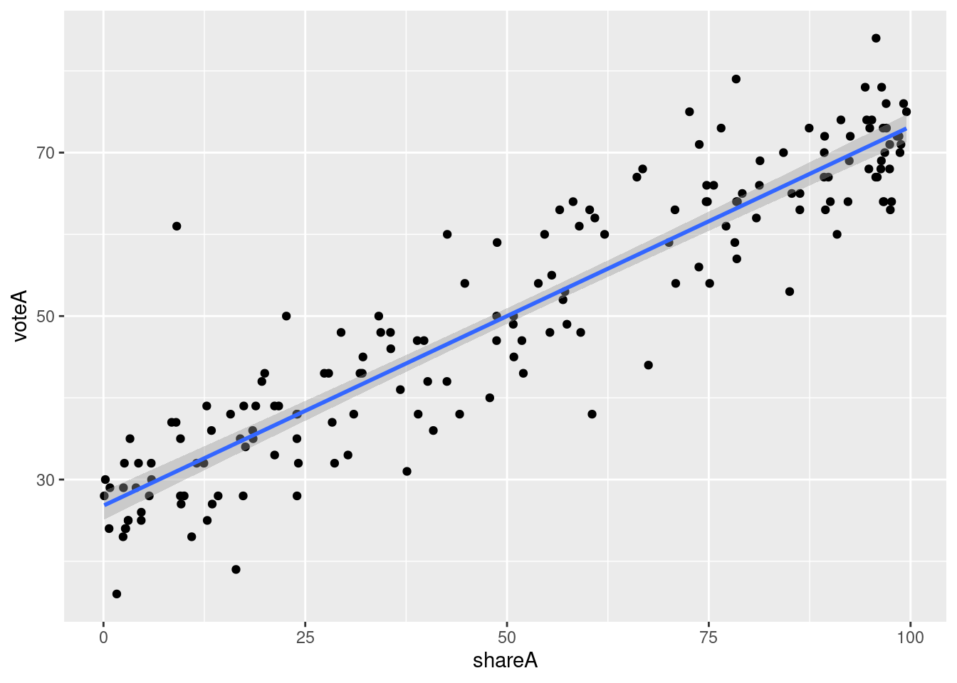
For \(\hat{\beta_1}\), display a sentence explaining how to calculate the t-stat and associated p-value, and displaying the widest standard (i.e., 90%, 95%, or 99%) confidence interval that does not contain 0 (with all values coming from inline r code, modeled after the sentence above for example 2.3):
The t-stat is calculated by dividing the estimated coefficient (0.464) by its standard error (0.0145), yielding a t-stat of 31.901 and an associated p-value of 6.63e-74; the widest standard confidence interval that does not include 0 is the 99% confidence interval: (0.426, 0.502).
10.5 Example of Fitted Values (\(\hat{y}\))
This example builds off of Example 2.3: CEO Salary and Return on Equity above. You don’t need to do anything for these, but you should look at them to make sure you understand them.
First, you should understand how to calculate the OLS fitted values, the \(\hat{y}\) values. Below you’ll see two ways to do so. The first is to manually use the OLS regression equation:
\[ \hat{y}_i = \hat{\beta}_0 + \hat{\beta}_1 x_i \]
After estimating a model, you can use the coef() function to get the values of \(\hat{\beta}_0\) and \(\hat{\beta}_1\).
We estimated the model above and stored it into the variable ex2.3. We can access \(\hat{\beta}_0\) with coef(ex2.3)["(Intercept)"] or coef(ex2.3)[1]. We can access the first (and only) \(x\) variable is named roe, and \(\hat{\beta}_1\) is coef(ex2.3)["roe"] or coef(ex2.3)[1].
The second way is by using the fitted() function.
You can check that these two are the same by subtracting them and making sure they are all the same.
##       Min.    1st Qu.     Median       Mean    3rd Qu.       Max.
## -2.046e-12  0.000e+00  0.000e+00  2.557e-14  0.000e+00  1.137e-12
Note that the min is -0.000000000002046363 and the max is 0.000000000001136868. Algebra with decimal numbers often results in small rounding errors, which is why these aren’t 0 exactly, but they are effectively 0, demonstrating that the two methods of calculating the fitted \((\hat{y})\) values are the same.
The second reason I’m including this example is to demonstrate plotting the fitted \((\hat{y})\) values. The black circles are the data. The red x’s are the predicted \((\hat{y})\) values (in this setting, “predicted values” and “fitted” values and \((\hat{y})\) all mean the same thing). The blue line is the OLS regression line. You should understand why all of the red x’s are on the blue line.
ggplot(data=ceosal1, aes(x=roe, y=salary)) +
  geom_point(aes(color="data",shape="data")) +
  geom_point(aes(x=roe, y=salaryHat,color="predicted (yHat)",shape="predicted (yHat)")) +
  geom_smooth(method = "lm",color="blue", se=FALSE,aes(linetype="OLS")) +
  scale_color_manual(values = c("black", "red"),name="Values") +
  scale_shape_manual(values = c(1,4),name="Values") +
  scale_linetype_manual(values = c("solid","solid"), name="Regression Line")
## `geom_smooth()` using formula = 'y ~ x'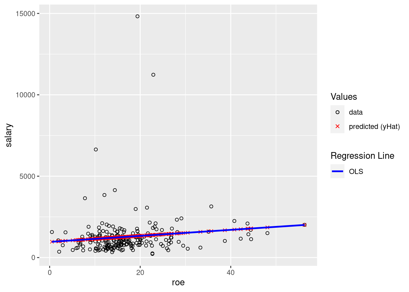
The 90%, 95%, and 99% confidence intervals are only “standard” because people typically like round numbers and have decided that these are the values typically reported. There is no statistical reason why as a society we couldn’t have decided to commonly discuss 92%, 97%, etc. But, 90%, 95%, and 99% are what are usually reported (and when we discuss the idea of statistical significance, we’ll discuss the corresponding 10%, 5%, and 1% “standard” levels of statistical significance).↩︎
Note that “review” can mean go back and look at things you’ve done in the past, e.g., what you did in STAT 255, but it can also mean learn/help yourself better understand things on your own. For example, Google confidence intervals and read some of what you find, watch videos, ask something like chatGPT, etc. Being able to learn/re-learn things on your own is a valuable long-term skill, and one you should practice with things like this.↩︎